hepi.plot
Module Contents
Functions
|
Sets the title on axis axe. |
|
Plot energy on the x-axis. |
|
|
|
|
|
Get the mass of particle with id iid out of the list in the "slha" element in the dict. |
|
Creates a plot based on the entries x`and `y in dict_list. |
|
|
|
|
|
|
|
Creates a plot based on the values in x`and `y. |
|
|
|
Examples |
|
Scatter map 2d. |
|
|
|
Creates a scale variance plot with 5 panels (xline). |
|
Creates a scale variance plot with 3 panels (ystacked). |
|
Initialze subplot for Ratio/K plots with another figure below. |
Attributes
- hepi.plot.title(i: hepi.input.Input, axe=None, scenario='', diff_L_R=None, extra='', cms_energy=True, pdf_info=True, id=False, **kwargs)[source]
Sets the title on axis axe.
- hepi.plot.energy_plot(dict_list, y, yscale=1.0, xaxis='E [GeV]', yaxis='$\\sigma$ [pb]', label=None, **kwargs)[source]
Plot energy on the x-axis.
- hepi.plot.mass_plot(dict_list, y, part, logy=True, yaxis='$\\sigma$ [pb]', yscale=1.0, label=None, **kwargs)[source]
- hepi.plot.mass_vplot(dict_list, y, part, logy=True, yaxis='$\\sigma$ [pb]', yscale=1.0, label=None, mask=None, **kwargs)[source]
- hepi.plot.get_mass(l: dict, iid: int)[source]
Get the mass of particle with id iid out of the list in the “slha” element in the dict.
- Returns
listof float : masses of particles in each element of the dict list.
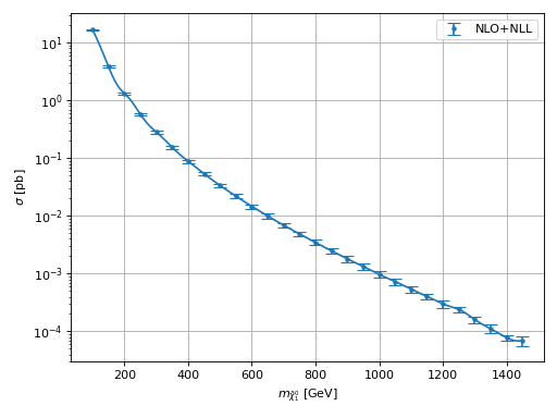
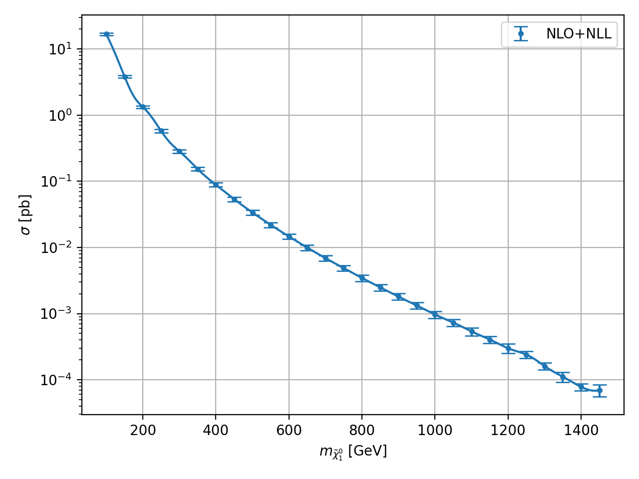
- hepi.plot.plot(dict_list, x, y, label=None, xaxis='E [GeV]', yaxis='$\\sigma$ [pb]', ratio=False, K=False, K_plus_1=False, logy=True, yscale=1.0, mask=None, **kwargs) None[source]
Creates a plot based on the entries x`and `y in dict_list.
Examples
>>> import urllib.request
>>> import hepi
>>> dl = hepi.load(urllib.request.urlopen(
... "https://raw.githubusercontent.com/fuenfundachtzig/xsec/master/json/pp13_hino_NLO%2BNLL.json"
... ))
>>> hepi.plot(dl,"N1","NLO_PLUS_NLL",xaxis="$m_{\\tilde{\\chi}_1^0}$ [GeV]")
(Source code, png, hires.png, pdf)
- hepi.plot.vplot(x, y, label=None, xaxis='E [GeV]', yaxis='$\\sigma$ [pb]', logy=True, yscale=1.0, interpolate=True, plot_data=True, data_color=None, mask=- 1, fill=False, data_fmt='.', fmt='-', print_area=False, sort=True, **kwargs)[source]
Creates a plot based on the values in x`and `y.
- hepi.plot.mass_mapplot(dict_list, part1, part2, z, logz=True, zaxis='$\\sigma$ [pb]', zscale=1.0, label=None)[source]
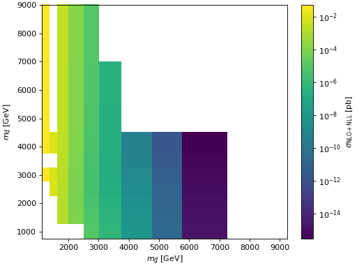
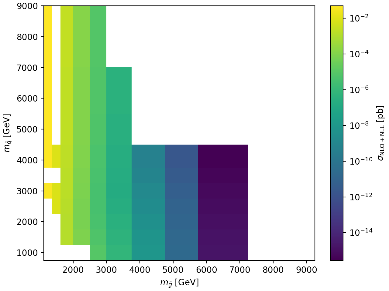
- hepi.plot.mapplot(dict_list, x, y, z, xaxis=None, yaxis=None, zaxis=None, **kwargs)[source]
Examples
>>> import urllib.request
>>> import hepi
>>> dl = hepi.load(urllib.request.urlopen(
... "https://raw.githubusercontent.com/APN-Pucky/xsec/master/json/pp13_SGmodel_GGxsec_NLO%2BNLL.json"
... ),dimensions=2)
>>> hepi.mapplot(dl,"gl","sq","NLO_PLUS_NLL",xaxis="$m_{\\tilde{g}}$ [GeV]",yaxis="$m_{\\tilde{q}}$ [GeV]" , zaxis="$\\sigma_{\\mathrm{NLO+NLL}}$ [pb]")
(Source code, png, hires.png, pdf)
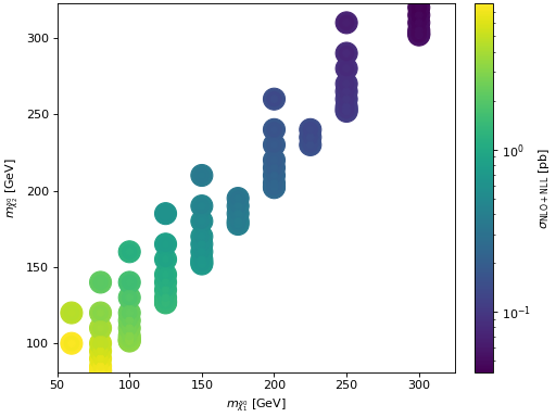
- hepi.plot.scatterplot(dict_list, x, y, z, xaxis=None, yaxis=None, zaxis=None, **kwargs)[source]
Scatter map 2d. Central color is the central value, while the inner and outer ring are lower and upper bounds of the uncertainty interval.
Examples
>>> import urllib.request
>>> import hepi
>>> dl = hepi.load(urllib.request.urlopen(
... "https://raw.githubusercontent.com/APN-Pucky/xsec/master/json/pp13_hinosplit_N2N1_NLO%2BNLL.json"
... ),dimensions=2)
>>> hepi.scatterplot(dl,"N1","N2","NLO_PLUS_NLL",xaxis="$m_{\\tilde{\\chi}_1^0}$ [GeV]",yaxis="$m_{\\tilde{\\chi}_2^0}$ [GeV]" , zaxis="$\\sigma_{\\mathrm{NLO+NLL}}$ [pb]")
(Source code, png, hires.png, pdf)
- hepi.plot.scale_plot(dict_list, vl, seven_point_band=False, cont=False, error=True, li=None, plehn_color=False, yscale=1.0, unit='pb', yaxis=None, **kwargs)[source]
Creates a scale variance plot with 5 panels (xline).